Tutorial
This tutorial demonstrates basic usage of the PyMGRIT package. Our goal is solving Dahlquist’s test problem,
discretized by Backward Euler. To accomplish this, this tutorial will go through the following tasks:
Writing the vector class holding all time-dependent information
Writing the application class holding any time-independent data
implementation: dahlquist.py (steps 1 and 2), example_dahlquist.py (step 3)
Vector class
The first step is to write a data structure that contains the solution of a single point in time. The data structure must inherit from PyMGRIT’s core Vector class.
For our test problem, we import PyMGRIT’s core Vector class (and numpy for later use):
import numpy as np
from pymgrit.core.vector import Vector
Then, we define the class VectorDahlquist containing a scalar member variable value:
class VectorDahlquist(Vector):
    """
    Vector class for Dahlquist's test equation
    """

    def __init__(self, value):
        super().__init__()
        self.value = value
Furthermore, we must define the following seven member functions: set_values, get_values, clone, clone_zero, clone_rand, __add__, __sub__, __mul__, norm, pack and unpack.
The function set_values receives data values and overwrites the values of the vector data and get_values returns the vector data. For our class VectorDahlquist, the vector data is the scalar member variable value:
def set_values(self, value):
    self.value = value

def get_values(self):
    return self.value
The function clone clones the object. The function clone_zero returns a vector object initialized with zeros; clone_rand similarly returns a vector object initialized with random data. For our class VectorDahlquist, these member functions are defined as follows:
def clone(self):
    return VectorDahlquist(self.value)

def clone_zero(self):
    return VectorDahlquist(0)

def clone_rand(self):
    return VectorDahlquist(np.random.rand(1)[0])
The functions __add__, __sub__, __mul__, and norm define the addition and subtraction of two vector objects and the norm of a vector object, respectively.
For our class VectorDahlquist, adding or subtracting two vector objects means adding or subtracting the values of the member variable value by using the functions get_values and set_values.
The multiplication defines the multiplication of a vector objects with a float.
We define the norm of a vector object as the norm (from numpy) of the member variable value:
def __add__(self, other):
    tmp = VectorDahlquist(0)
    tmp.set_values(self.get_values() + other.get_values())
    return tmp

def __sub__(self, other):
    tmp = VectorDahlquist(0)
    tmp.set_values(self.get_values() - other.get_values())
    return tmp

def __mul__(self, other):
    tmp = VectorDahlquist(0)
    tmp.set_values(self.get_values() * other)
    return tmp

def norm(self):
    return np.linalg.norm(self.value)
The functions pack and unpack define the data to be communicated and how data is unpacked after receiving it. For our class VectorDahlquist, packing means setting the data to be communicated to the member variable value and unpacking means setting the member variable value to the received scalar value:
def pack(self):
    return self.value

def unpack(self, value):
    self.value = value
Summary
The vector class must inherit from PyMGRIT’s core Vector class.
Member variables hold all data of a single time point.
The following member functions must be defined:
set_values : Setting vector data
get_values : Getting vector data
clone : Initialization of vector data with equivalent values
clone_zero : Initialization of vector data with zeros
clone_rand : Initialization of vector data with random values
__add__ : Addition of two vector objects
__sub__ : Subtraction of two vector objects
__mul__ : Multiplication of a vector object with a float
norm : Norm of a vector object (for measuring convergence)
pack : Specifying communication data
unpack : Unpacking communication data
import numpy as np
from pymgrit.core.vector import Vector

class VectorDahlquist(Vector):
    """
    Vector class for Dahlquist's test equation
    """

    def __init__(self, value):
        super().__init__()
        self.value = value

    def set_values(self, value):
        self.value = value

    def get_values(self):
        return self.value

    def clone(self):
        return VectorDahlquist(self.value)

    def clone_zero(self):
        return VectorDahlquist(0)

    def clone_rand(self):
        return VectorDahlquist(np.random.rand(1)[0])

    def __add__(self, other):
        tmp = VectorDahlquist(0)
        tmp.set_values(self.get_values() + other.get_values())
        return tmp

    def __sub__(self, other):
        tmp = VectorDahlquist(0)
        tmp.set_values(self.get_values() - other.get_values())
        return tmp

    def __mul__(self, other):
        tmp = VectorDahlquist(0)
        tmp.set_values(self.get_values() * other)
        return tmp

    def norm(self):
        return np.linalg.norm(self.value)

    def pack(self):
        return self.value

    def unpack(self, value):
        self.value = value
Application class
In the next step we write the application class that contains information about the problem we want to solve. Every application class must inherit from PyMGRIT’s core Application class.
For our test problem, we import PyMGRIT’s core Application class:
from pymgrit.core.application import Application
Then, we define the class Dahlquist containing the member variable vector_template that defines the data structure for any user-defined time point as well as the member variable vector_t_start that holds the initial condition at time t_start:
class Dahlquist(Application):
    """
    Application class for Dahlquist's test equation,
       u' = lambda u,  u(0) = 1,
    with lambda = -1
    """

    def __init__(self, *args, **kwargs):
        super().__init__(*args, **kwargs)

        # Set the data structure for any user-defined time point
        self.vector_template = VectorDahlquist(0)

        # Set the initial condition
        self.vector_t_start = VectorDahlquist(1)
Note: The time interval of the problem is defined in the superclass Application. This PyMGRIT core class contains the following member variables:
t_start : start time (left bound of time interval)
t_end : end time (right bound of time interval)
nt : number of time points
Furthermore, we must define the time integration routine as the member function step that evolves a vector u_start from time t_start to time t_stop. For our test problem, we take a backward Euler step:
def step(self, u_start: VectorDahlquist, t_start: float, t_stop: float) -> VectorDahlquist:
    z = (t_stop - t_start) * -1  # Note: lambda = -1
    tmp = 1 / (1 - z) * u_start.get_values()
    return VectorDahlquist(tmp)
Summary
The application class must inherit from PyMGRIT’s core Application class.
The application class contains information about the problem we want to solve.
The application class must contain the following member variables and member functions:
Variable vector_template : Data structure for any user-defined time point
Variable vector_t_start : Holds the initial condition (same data structur as vector_template)
Function step : Time integration routine
# Import superclass Application
from pymgrit.core.application import Application

class Dahlquist(Application):
    """
    Application class for Dahlquist's test equation,
       u' = lambda u,  u(0) = 1,
    with lambda = -1
    """

    def __init__(self, *args, **kwargs):
        super().__init__(*args, **kwargs)

        # Set the data structure for any user-defined time point
        self.vector_template = VectorDahlquist(0)

        # Set the initial condition
        self.vector_t_start = VectorDahlquist(1)

    # Time integration routine
    def step(self, u_start: VectorDahlquist, t_start: float, t_stop: float) -> VectorDahlquist:
        z = (t_stop - t_start) * -1  # Note: lambda = -1
        tmp = 1 / (1 - z) * u_start.get_values()
        return VectorDahlquist(tmp)
Solving the problem
The third step is to set up an MGRIT solver for the test problem.
First, import PyMGRIT:
from pymgrit import *
Create Dahlquist’s test problem for the time interval [0, 5] with 101 equidistant time points (100 time points + 1 time point for the initial time t = 0) as an object of our application class Dahlquist:
dahlquist = Dahlquist(t_start=0, t_stop=5, nt=101)
Construct a multigrid hierarchy for the test problem dahlquist using PyMGRIT’s core function simple_setup_problem:
dahlquist_multilevel_structure = simple_setup_problem(problem=dahlquist, level=2, coarsening=2)
This tells PyMGRIT to set up a hierarchy with two temporal grid levels using the test problem dahlquist and a temporal coarsening factor of two, i.e., on the fine grid, the number of time points is 101, and on the coarse grid, 51 (=100/2+1) time points are used.
Set up the MGRIT solver for the test problem using dahlquist_multilevel_structure and set the solver tolerance to 1e-10:
mgrit = Mgrit(problem=dahlquist_multilevel_structure, tol=1e-10)
which produces the output:
INFO - 03-02-20 11:19:03 - Start setup
INFO - 03-02-20 11:19:03 - Setup took 0.009920358657836914 s
Finally, solve the test problem using the solve() routine of the solver mgrit:
info = mgrit.solve()
which gives:
INFO - 03-02-20 11:19:03 - Start solve
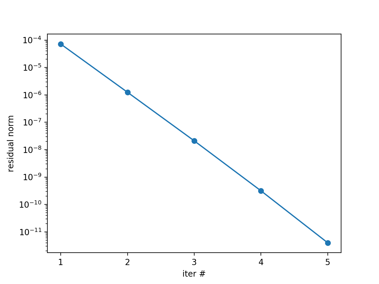
INFO - 03-02-20 11:19:03 - iter 1 | conv: 7.186185937031941e-05 | conv factor: - | runtime: 0.01379704475402832 s
INFO - 03-02-20 11:19:03 - iter 2 | conv: 1.2461067076355103e-06 | conv factor: 0.017340307063501627 | runtime: 0.007235527038574219 s
INFO - 03-02-20 11:19:03 - iter 3 | conv: 2.1015566145245807e-08 | conv factor: 0.016864981158092696 | runtime: 0.005523681640625 s
INFO - 03-02-20 11:19:03 - iter 4 | conv: 3.144127445017594e-10 | conv factor: 0.014960945726074891 | runtime: 0.004599332809448242 s
INFO - 03-02-20 11:19:03 - iter 5 | conv: 3.975214076032893e-12 | conv factor: 0.01264329816633959 | runtime: 0.0043201446533203125 s
INFO - 03-02-20 11:19:03 - Solve took 0.042092084884643555 s
INFO - 03-02-20 11:19:03 - Run parameter overview
interval : [0.0, 5.0]
number points : 101 points
max dt : 0.05000000000000071
level : 2
coarsening : [2]
cf_iter : 1
nested iteration : True
cycle type : V
stopping tolerance : 1e-10
communicator size time : 1
communicator size space : 1
and returns the residual history, setup time, and solve time in dictionary info with the following key values:
conv : residual history (2-norm of the residual at each iteration)
time_setup : setup time [in seconds]
time_solve : solve time [in seconds]
Summary
# Import PyMGRIT
from pymgrit import *

# Create Dahlquist's test problem with 101 time steps in the interval [0, 5]
dahlquist = Dahlquist(t_start=0, t_stop=5, nt=101)

# Construct a two-level multigrid hierarchy for the test problem using a coarsening factor of 2
dahlquist_multilevel_structure = simple_setup_problem(problem=dahlquist, level=2, coarsening=2)

# Set up the MGRIT solver for the test problem and set the solver tolerance to 1e-10
mgrit = Mgrit(problem=dahlquist_multilevel_structure, tol=1e-10)

# Solve the test problem
info = mgrit.solve()
Looking at results
The last step is to look at the results of our PyMGRIT run.
In the default setting,
PyMGRIT’s core routine Mgrit() prints out the setup time.
The solve() routine
prints out the residual history, along with convergence factors and runtimes, and
returns the residual history, setup time, and solve time.
For our example, we can plot the residuals as follows: First, we import numpy and pyplot:
import numpy as np
import matplotlib.pyplot as plt
Then, we get the residuals from the dictionary info:
res = info['conv']
and plot the residuals:
iters = np.arange(1, res.size+1)
plt.semilogy(iters, res, 'o-')
plt.xticks(iters)
plt.xlabel('iter #')
plt.ylabel('residual norm')
plt.show()
which gives
Summary
import numpy as np
import matplotlib.pyplot as plt

from pymgrit import *

# Create Dahlquist test problem and solve resulting linear system using a two-level MGRIT solver
dahlquist = Dahlquist(t_start=0, t_stop=5, nt=101)
dahlquist_multilevel_structure = simple_setup_problem(problem=dahlquist, level=2, coarsening=2)
mgrit = Mgrit(problem=dahlquist_multilevel_structure, tol=1e-10)
info = mgrit.solve()

# Plot the residual history
res = info['conv']
iters = np.arange(1, res.size+1)
plt.semilogy(iters, res, 'o-')
plt.xticks(iters)
plt.xlabel('iter #')
plt.ylabel('residual norm')
plt.show()