Parallelism¶

This page contains short examples that demonstrate the parallel usage of PyMGRIT.

Time parallelism

Space & time parallelism

Time parallelism¶

Use mpirun to run an example in parallel:

>>> mpiexec -np 2 python3 example_dahlquist.py

Output function¶

example_output_fcn.py

In this example, we show how to use the output function for a parallel run and save the solution after each iteration. Each process calls the function, so the file of each process must be unique. We use the rank to distinguish the files. We save the solution and the time point in a list for each local point of one process:

def output_fcn(self):
    # Set path to solution; here, we include the iteration number in the path name
    path = 'results/' + 'brusselator' + '/' + str(self.solve_iter)
    # Create path if not existing
    pathlib.Path(path).mkdir(parents=True, exist_ok=True)

    # Save solution to file.
    # Useful member variables of MGRIT solver:
    #   - self.t[0]           : local fine-grid (level 0) time interval
    #   - self.index_local[0] : indices of local fine-grid (level 0) time interval
    #   - self.u[0]           : fine-grid (level 0) solution values
    #   - self.comm_time_rank : Time communicator rank
    np.save(path + '/brusselator-rank' + str(self.comm_time_rank),
            [[[self.t[0][i], self.u[0][i]] for i in self.index_local[0]]])  # Solution and time at local time points

Then, we solve the problem in the usual way:

# Create two-level time-grid hierarchy for the Brusselator system
brusselator_lvl_0 = Brusselator(t_start=0, t_stop=12, nt=641)
brusselator_lvl_1 = Brusselator(t_interval=brusselator_lvl_0.t[::20])

# Set up the MGRIT solver using the two-level hierarchy and set the output function
mgrit = Mgrit(problem=[brusselator_lvl_0, brusselator_lvl_1], output_fcn=output_fcn, output_lvl=2, cf_iter=0)

# Solve Brusselator system
info = mgrit.solve()

The last step is to plot the solution for each iteration. Therefore, all files have to be loaded and the solution has to be assembled in the correct order. To determine the correct order, we use the corresponding time points:

# Plot the MGRIT approximation of the solution after each iteration
if MPI.COMM_WORLD.Get_rank() == 0:
    # Dynamic images
    iterations_needed = len(info['conv']) + 1
    cols = 2
    rows = iterations_needed // cols + iterations_needed % cols
    position = range(1, iterations_needed + 1)
    fig = plt.figure(1, figsize=[10, 10])
    for i in range(iterations_needed):
        # Load each file and add the loaded values to sol
        sol = []
        path = 'results/brusselator/' + str(i)
        for filename in os.listdir(path):
            data = np.load(path + '/' + filename, allow_pickle=True).tolist()[0]
            sol += data
        # Sort the solution list by the time
        sol.sort(key=lambda tup: tup[0])
        # Get the solution values
        values = np.array([i[1].get_values() for i in sol])
        ax = fig.add_subplot(rows, cols, position[i])
        # Plot the two solution values at each time point
        ax.scatter(values[:, 0], values[:, 1])
        ax.set(xlabel='x', ylabel='y')
    fig.tight_layout(pad=2.0)
    plt.show()

Scaling results¶

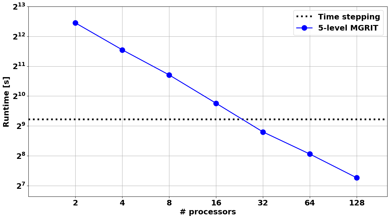
In the following we present strong scaling results for applying a five-level MGRIT V-cycle solver with FCF-relaxation and nested iterations to a 2D heat equation example. The problem setup is as follows:

Space-time domain: \([0, 1] \times [0, 1] \times [0, 5]\)
Thermal conductivity: \(a = 1\)
Right-hand side: \(b(x,y,t) = -\sin(x) * \sin(y) * (\sin(t) - 2 * \cos(t))\)
Homogeneous Dirichlet boundary conditions in space
Initial condition: \(u(x,y,0) = 0\)
Discretization:
- centered finite differences in space
- backward Euler in time
- discrete problem size: \(101 \times 51 \times 8193\)
5-level MGRIT V-cycles with FCF-relaxation and nested iterations
Coarsening strategy:
- factor-8 coarsening on finest level
- factor-4 coarsening on all coarse levels

Source code:

import numpy as np
from pymgrit.heat.heat_2d import Heat2D
from pymgrit.core.mgrit import Mgrit

def rhs(x, y, t):
    return -np.sin(x) * np.sin(y) * (np.sin(t) - 2 * np.cos(t))

heat0 = Heat2D(x_start=0, x_end=1, y_start=0, y_end=1, nx=101, ny=51, a=1, rhs=rhs, t_start=0, t_stop=5,
               nt=2 ** 13 + 1)
heat1 = Heat2D(x_start=0, x_end=1, y_start=0, y_end=1, nx=101, ny=51, a=1, rhs=rhs, t_interval=heat0.t[::8])
heat2 = Heat2D(x_start=0, x_end=1, y_start=0, y_end=1, nx=101, ny=51, a=1, rhs=rhs, t_interval=heat1.t[::4])
heat3 = Heat2D(x_start=0, x_end=1, y_start=0, y_end=1, nx=101, ny=51, a=1, rhs=rhs, t_interval=heat2.t[::4])
heat4 = Heat2D(x_start=0, x_end=1, y_start=0, y_end=1, nx=101, ny=51, a=1, rhs=rhs, t_interval=heat3.t[::4])

mgrit = Mgrit(problem=[heat0, heat1, heat2, heat3, heat4]).solve()

The parallel tests were performed on an Intel Xeon Phi Cluster consisting of 272 1.4 GHz Intel Xeon Phi processors.
Between two and 128 processors were used for parallelization in time
Runtimes are compared to sequential time-stepping

Total (setup + solve) runtimes:

Space & time parallelism¶

To be done.